
Overview
The Wasserstein distance (earth mover’s distance) measures how much “work” is needed to reshape one probability distribution into another. Unlike a change in volatility alone, it is sensitive to the whole shape of the return distribution: scale, skew and tail weight. In this study it is used as a relative change detector (a regime-shift signal) on EURUSD one-minute returns, not as a measure of market depth. Foreign exchange is decentralised, and retail tick volume covers well under 1% of daily turnover, so absolute order-book depth cannot be reconstructed from the data available to us.
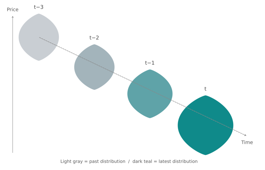
Why FX depth cannot be observed
The picture above says what we want to detect: the distribution of returns changes. Why not look at market depth directly, the amount that can be traded before the price moves? Because in foreign exchange that quantity is not observable. A stock trades on an exchange with one central order book, so anyone can see the resting size at each price and the volume actually traded. FX is an over-the-counter market: banks, dealers, electronic venues and non-bank liquidity providers each keep their own book, and there is no consolidated tape. The scale is large (the BIS Triennial Survey put global FX turnover at $9.6 trillion per day in April 2025, BIS press release), yet no participant sees all of it.
What a retail data feed gives is a bid and ask price per minute and, at best, a tick count. A tick count is the number of quote updates, not the amount traded, so it is a weak stand-in for volume. Even the depth a venue displays is not firm: liquidity providers can use last look to reject a trade, keep part of their size hidden, or pull quotes just before news. The displayed size therefore overstates what can really be traded exactly when it matters most.
Depth therefore shows up only through its effects, and the most direct one is the distribution of returns. When depth thins, the same flow moves the price further, so returns become larger, more dispersed and more jumpy. That is why this article compares return distributions instead of measuring depth, and why the output is a relative signal, meaning this window differs from the previous one, and not an absolute liquidity gauge.
This approach has a clear limit. A thinner book and a burst of news both widen the distribution, and the detector cannot tell the two apart. It signals that the regime changed but says nothing about the cause. The event study below shows how much of the signal lines up with scheduled releases and how much does not.
Mathematical Formulation
For two one-dimensional distributions with quantile functions F⁻¹ and G⁻¹, the first-order Wasserstein distance is W₁ = ∫₀¹ |F⁻¹(u) − G⁻¹(u)| du. For two equal-size samples this reduces to the mean absolute difference of the sorted values: W₁ = mean |sort(a) − sort(b)|. The barycenter (the “average distribution” used as a cluster centre in Wasserstein K-means) is the mean of the quantile functions. Multi-dimensional cases require optimal-transport solvers (e.g. Sinkhorn iterations); the 1-D case needs only a sort.
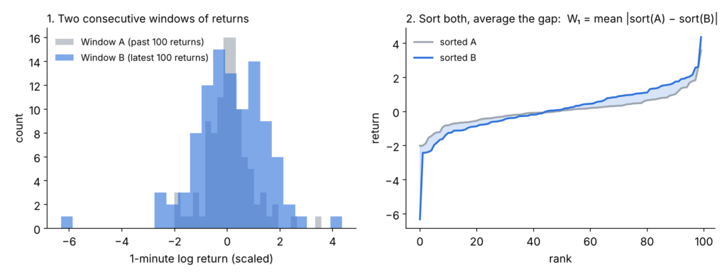
Redistribution cost: how W1 is computed
Think of each return distribution as a pile of earth: every observation is one equal unit of earth, lying at its return value. The Wasserstein distance is the least total work needed to reshape pile A into pile B, where moving earth costs (amount moved) × (distance moved). Distance is measured in return units, so the result is directly readable: if every return of A is shifted by δ to give B, then W1 = |δ|.
For two samples of the same size n the cheapest plan is always to match them in rank order: the smallest value of A goes to the smallest of B, the second smallest to the second smallest, and so on. Any plan that crosses these pairs costs at least as much. The cost of the sorted plan is the mean of the absolute gaps between matched values.
W1 = (gap 1 + gap 2 + … + gap n) / n, where gap i is the absolute difference between the i-th smallest value of A and the i-th smallest value of B.
A worked example with five returns, in basis points (0.01%): A = {0.1, −0.2, 0.0, 0.3, −0.1} and B = {0.8, −0.3, 0.1, −0.5, 0.4}. Sorted, the pairs and their moving distances are:
| Rank | Sorted A | Sorted B | Distance moved |
|---|---|---|---|
| 1 | −0.2 | −0.5 | 0.3 |
| 2 | −0.1 | −0.3 | 0.2 |
| 3 | 0.0 | 0.1 | 0.1 |
| 4 | 0.1 | 0.4 | 0.3 |
| 5 | 0.3 | 0.8 | 0.5 |
| Total / mean | 1.4 / 0.28 |
So W1 = 0.28 bp. Pairing the observations in time order instead (0.1 with 0.8, −0.2 with −0.3, and so on) would cost 0.44 bp on average, more than the sorted plan, which is why the sort is part of the definition. In the detector, A is the previous 100 one-minute returns and B the latest 100; the absolute size of W1 has no meaning by itself, which is why it is then standardised with a rolling z-score.
Three properties matter for this use. First, it works directly on the raw samples, with no histogram or density estimate, and the cost is that of a sort (n log n), cheap enough to run at every minute of fourteen years of data. Second, it measures how far the mass has to move: scaling all returns by a factor s costs the absolute value of (s − 1) times the mean absolute return, so the same number reacts to changes in volatility as well as to changes in skew and tails, and a few extreme returns weigh more than many small moves near zero. Third, divergences such as KL need overlapping density estimates and say nothing about how far apart two distributions are, whereas W1 stays finite and meaningful even when they barely overlap. For several dimensions there is no sort shortcut and the cost has to be solved as a transport problem, usually approximated with the Sinkhorn algorithm; the 1D case used here is the exception where it is exact and cheap.
Application: A Rolling Detector
- Data: EURUSD M1 bid (Dukascopy). Development period 2019-01-01 to 2026-09-05 (3,383,371 bars); out-of-sample period 2012-01-01 to 2018-12-31 (3,092,918 bars). Log returns are clipped at a fixed level of 0.000873, the 99.9th percentile of |r| in the development period. These files list every minute, so minutes without any trade appear as flat bars (about 22% of returns are exactly zero). GBPUSD, USDJPY, AUDUSD and XAUUSD come from the same vendor and format (2012-01-01 to 2026-10-30).
- At each bar t, take two consecutive, non-overlapping windows of 100 returns and compute W₁ between them.
- Standardise W₁ with a rolling z-score (lookback 1,000 bars). Flag a regime shift when z > 2.0.
- Rollover artifact: around 21:00–22:00 UTC the price is nearly flat, which produced spurious extreme values. Windows with fewer than 50 non-zero returns in either half are excluded.
Empirical Check Against Scheduled Macro Events
As a sanity test, we checked whether the detector reacts to events that are known to move EURUSD: FOMC decisions, US Non-Farm Payrolls, US CPI and ECB monetary-policy decisions. US release dates were taken from the BLS release calendars (including holiday and government-shutdown rescheduling) and converted to UTC with the correct daylight-saving offset. ECB dates are all scheduled monetary-policy meetings, timed at the release of the rate decision (13:45 Frankfurt time until the July 2022 meeting, 14:15 from the 21 July 2022 meeting on, when the ECB moved its announcement). An event counts as detected if at least one flagged bar occurs within ±60 minutes. As a control, each event was compared with the same weekday and clock time in other weeks that contain no event.
Development period, 2019–2026 (306 events)
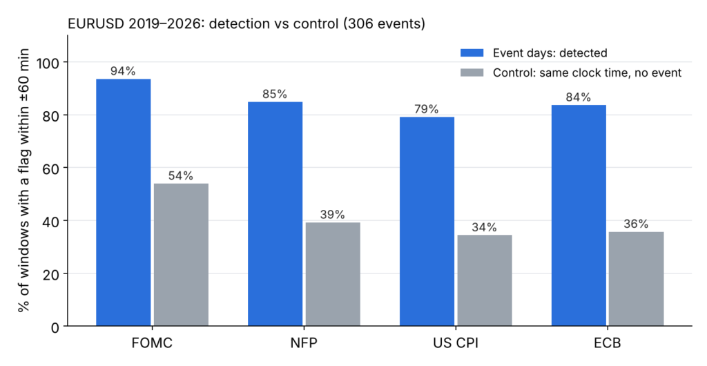
| Event | Events | Detected | Control (same clock time, non-event weeks) |
|---|---|---|---|
| FOMC | 62 | 93.5% | 53.9% |
| NFP | 92 | 84.8% | 39.2% |
| CPI | 91 | 79.1% | 34.4% |
| ECB | 61 | 83.6% | 35.7% |
| All | 306 | 84.6% | 40.1% |
Precision: 6.58% of all flagged bars fall within ±60 minutes of a listed event, versus 1.50% of all valid bars that lie in such a window, a lift of about 4.4x. Of the 47 undetected events, 12 were near-misses (peak z between 1.5 and 2.0), 21 produced little distributional reaction, and 14 had no usable data in the window.
Out-of-sample period, 2012–2018 (292 events)
The detector and all parameters were left unchanged and applied to the earlier seven years, which were not used when the settings were chosen.
| Event | Events | Detected | Control (same clock time, non-event weeks) |
|---|---|---|---|
| FOMC | 56 | 89.3% | 52.1% |
| NFP | 84 | 97.6% | 45.4% |
| CPI | 84 | 66.7% | 33.5% |
| ECB | 68 | 80.9% | 23.0% |
| All | 292 | 83.2% | 38.3% |
Precision was 5.95% against a 1.60% coverage baseline (about 3.7x), and the detector flagged 7.7% of bars with a valid score, the same as in the development period. The pattern is the same: NFP and FOMC are detected most reliably, then ECB decisions and CPI, with a median peak z of 3.9 for ECB and 2.8 for CPI versus 5.1 to 5.6 for FOMC and NFP. The lift over the control is about 2.2x overall (3.5x for ECB), against 2.1x in 2019–2026, so the effect does not look specific to the development period.
Continuous 2012–2026 run. A single EURUSD file covering 2012-01-01 to 2026-10-30 (all-minutes format, same as above) was also run as one uninterrupted series, restricted to the same 598 events (292 + 306, up to 2026-09-05). The 2012–2018 and 2019–2026 subsets reproduce the figures above (83.2% and 84.6% detected). Over all 598 events the detection rate is 83.9% against a control of 39.2% (a lift of 2.1x), with precision 6.27% against a 1.55% coverage baseline (4.0x). By type: FOMC 91.5% vs 52.8%, NFP 90.9% vs 42.1%, US CPI 73.1% vs 34.0%, ECB 82.2% vs 28.9%.
Other instruments
The same detector (same window, lookback, threshold and activity filter) was run on four more instruments, against the same list of US and ECB events. Each instrument was run as one continuous file covering 2012-01-01 to 2026-10-30 in the all-minutes format used for EURUSD, so the rows are directly comparable; events are the same 598 up to 2026-09-05. Only the return clipping level was set per instrument, at the 99.9th percentile of |r| in its own data, because price scales differ (EURUSD keeps its fixed level). Each cell shows the detection rate and the same-clock-time control, in percent.
2012–2026, all 598 events
| Instrument | All (detected / control) | NFP | FOMC | US CPI | ECB | Precision vs coverage |
|---|---|---|---|---|---|---|
| EURUSD | 83.9 / 39.2 | 90.9 / 42.1 | 91.5 / 52.8 | 73.1 / 34.0 | 82.2 / 28.9 | 6.27% vs 1.55% |
| GBPUSD | 73.4 / 37.5 | 92.6 / 36.0 | 82.2 / 46.4 | 57.1 / 34.4 | 61.2 / 35.3 | 5.28% vs 1.56% |
| USDJPY | 74.2 / 32.7 | 92.0 / 31.5 | 89.8 / 47.7 | 66.3 / 29.4 | 46.5 / 25.1 | 5.65% vs 1.55% |
| AUDUSD | 72.4 / 31.9 | 93.8 / 37.3 | 93.2 / 52.3 | 63.4 / 21.4 | 36.4 / 19.0 | 5.33% vs 1.55% |
| XAUUSD* | 82.3 / 56.8 | 94.9 / 65.8 | 89.8 / 51.6 | 80.6 / 60.3 | 60.5 / 44.5 | 5.75% vs 1.56% |
Detection rate by period (all events)
| Instrument | 2012–2018 (292 events) | 2019–2026 (306 events) |
|---|---|---|
| EURUSD | 83.2% | 84.6% |
| GBPUSD | 67.5% | 79.1% |
| USDJPY | 70.9% | 77.5% |
| AUDUSD | 70.2% | 74.5% |
| XAUUSD* | 82.2% | 82.4% |
Local central-bank decisions (each pair’s own region)
| Instrument | Central bank (time used) | Events | All (detected / control) | 2012–2018 | 2019–2026 |
|---|---|---|---|---|---|
| GBPUSD | Bank of England (12:00 London) | 136 | 48.5 / 23.7 | 57.3 / 28.5 | 37.7 / 17.7 |
| AUDUSD | Reserve Bank of Australia (14:30 Sydney) | 153 | 62.7 / 35.6 | 72.7 / 43.4 | 52.6 / 27.6 |
| USDJPY | Bank of Japan (12:00 Tokyo, assumed) | 142 | 37.3 / 22.2 | 40.0 / 22.3 | 33.9 / 21.9 |
These are all scheduled policy decisions of the central bank of each pair’s non-US currency, up to 2026-09-05, with the same detector and the same control method (weeks without any listed event, so US and ECB days are excluded from the control). They are separate from the US/ECB table above, which is unchanged. Bank of England and Reserve Bank of Australia decisions are detected about 2.0x and 1.8x as often as the control; their absolute rates (48% and 63%) are lower than for NFP or FOMC, and lower in 2019–2026 than in 2012–2018. The Bank of Japan result should not be relied on: the BoJ does not publish a fixed announcement time, only that the meeting ends around midday, and the lift over the control depends strongly on the time assumed (0.8x at 11:00, 1.0x at 11:30, 1.7x at 12:00, 2.7x at 13:00 and 3.5x at 13:30 Tokyo time), partly because the control rate itself changes with clock time. The 12:00 value is shown only as a neutral midpoint, and a proper test needs the actual release time of each decision. Unscheduled decisions in March 2020 (Bank of England, RBA) are not included.
Every instrument is detected above its control for every event type. The lift over the control is about 2.2x to 2.9x for NFP on the four currency pairs, 1.7x to 1.9x for FOMC on all five, and 1.7x to 3.0x for US CPI on the currency pairs (AUDUSD highest, GBPUSD lowest). For ECB decisions the lift is largest on EURUSD (2.8x, 82% detected) and about 1.7x to 1.9x on the other three pairs, where detection falls to 36–61%. Gold’s control rate is already 57% at these clock times, which limits its lift to about 1.3x to 1.7x. Detection is higher in 2019–2026 than in 2012–2018 for all five instruments, though for gold only marginally. Decisions of the Bank of England, Reserve Bank of Australia and Bank of Japan are covered in the separate table above. *Gold: the rolling z-score was computed from at least 500 valid values within the 1,000-bar lookback instead of all 1,000, because gold’s thin daily period leaves too few unbroken stretches. With the strict rule only about 16% of bars received a z-score and the detection rate was far lower. The relaxed rule gives results in line with earlier runs of gold on a different data export.
The detection rate on its own overstates the result: the detector flags about 5.3% of all bars (7.7% of bars with a valid score), and a flag can persist for up to 100 bars after a shift, so even ordinary times at the same clock time are flagged 32–57% of the time (all instruments pooled over event types). The informative number is the lift over the control, not the headline detection rate.
Limitations
- Not a trading signal. W₁ measures that the return distribution changed, not in which direction. No profitability claim is made.
- Parameters and periods. The parameters (window 100, lookback 1,000, threshold 2.0) were chosen by reasoning and one corrective step (the rollover filter), not by systematic optimisation, but they were set while looking at the first EURUSD file (2019–2026). The 2012–2018 EURUSD results and the other instruments were not used to adjust them. The one later change is the relaxed z-score rule for gold described above.
- Data format. All tables use one data format: exports that list every minute, with flat bars for minutes without trades (about 22% of returns are exactly zero). Another export that omits those minutes gives modestly different numbers (EURUSD 2019–2026: 75.8% against 79.1% detected over the same events, measured with the earlier ECB timing), so results should only be compared within one format. Gold in particular is sensitive to how the rolling z-score is computed in the all-minutes format.
- High base rate. A z-score threshold of 2 flags a large share of bars, which is why a control comparison is necessary.
- Event-time tolerance. The ±60 minute window is generous; shorter windows will lower detection rates, and the result depends on the event time being exact. An earlier version of this study timed ECB decisions at 13:15 Frankfurt time, 30 minutes before the actual rate announcement (13:45) and 60 minutes before it after July 2022 (14:15). That put the announcement at or beyond the edge of the window and understated ECB detection (EURUSD 2012–2026: 38% against 82% with the correct times). The ECB figures above use the correct announcement times; the US events use the official release times. The same sensitivity makes the Bank of Japan result unreliable, because the BoJ publishes no fixed release time.
- Calendar accuracy. US dates come from BLS calendars. ECB dates (all scheduled monetary-policy meetings, 2012–2026) were checked against the European Central Bank’s own published calendars and match. Bank of Japan and Reserve Bank of Australia dates come from their published meeting and decision lists; Bank of England dates come from its published MPC dates, except 2012–2014, which were taken as the Thursday of each meeting week in the published minutes list, and 2025, which uses the dates announced in advance. FOMC dates are decision days, and one emergency meeting (March 2020) is included. Other unscheduled central-bank actions (for example the ECB’s, Bank of England’s and RBA’s emergency actions in March 2020) are not included. Events after 2026-09-05 are not included. A first version of this analysis used an approximate NFP calendar; the figures above replace it.
- Tick volume is a proxy. Returns are from one data vendor and cannot represent total market liquidity.
Related
Math Models · Wavelet Transform · Kalman Filter · ARIMA · GARCH · Methodology